tags
#Statistics #Data Science #Machine Learning #Artificial Intelligence.
Statistics vs. Probability
What’s the difference?
- All use data to gather insight and ultimately make decisions
- Statistics is at the core of the data processing part
- Nowadays, computational aspects play an important role as data becomes larger
Computational and statistical aspects of data science
- Computational view: data is a (large) sequence of numbers that needs to be processed by a relatively fast algorithm: approximate nearest neighbors, low dimensional embeddings, spectral methods, distributed optimization, etc.
- Statistical view: data comes from a random process. The goal is to learn how this process works in order to make predictions or to understand what plays a role in it. To understand randomness, we need Probability.
Probability
- Probability studies randomness (hence the prerequisite)
- Sometimes, the physical process is completely known: dice, cards, roulette, fair coins, . . .
- Rolling 1 die:
- Alice gets $1 if # of dots 3
- I Bob gets $2 if # of dots 2
- Who do you want to be: Alice or Bob?
- Rolling 2 dice:
- Choose a number between 2 and 12
- Win $100 if you chose the sum of the 2 dice
- Which number do you choose?
- Rolling 1 die:
Statistics and modeling
- Dice are well known random process from physics: 1/6 chance of each side (no need for data!), dice are independent. We can deduce the probability of outcomes, and expected $ amounts. This is probability.
- How about more complicated processes? Need to estimate parameters from data. This is statistics.
- Sometimes real randomness (ra
- ndom student, biased coin, measurement error, . . . )
- Sometimes deterministic but too complex phenomenon: statistical modeling Complicated process “=” Simple process + random noise
- (good) Modeling consists in choosing (plausible) simple process and noise distribution.
- 우리가 알 수 없는 random noise는 최소화하고, simple process 를 최대화해야함.
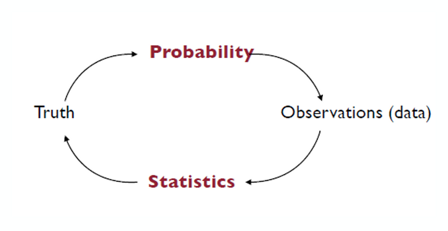
Statistics vs. Probability
- Probability Previous studies showed that the drug was 80% effective. Then we can anticipate that for a study on 100 patients, in average 80 will be cured and at least 65 will be cured with 99.99% chances.
- Statistics Observe that 78/100 patients were cured. We (will be able to) conclude that we are 95% confident that for other studies the drug will be effective on between 69.88% and 86.11% of patients.
→ 확률은 결과를 예측/추론 하는 것이고, 통계는 관찰을 바탕으로 모수를 추정하는 것
Statistical experiment
“A neonatal right-side preference makes a surprising romantic reappearance later in life.”
- Let $p$ denote the proportion of couples that turn their head to the right when kissing.
- Let us design a statistical experiment and analyze its outcome.
- Observe n kissing couples times and collect the value of each outcome (say 1 for RIGHT and 0 for LEFT)
- Estimate p with the proportion p_hat of RIGHT.
- Study: “Human behaviour: Adult persistence of head-turning asymmetry” (Nature, 2003): n = 124 and 80 to the right so p_hat= 64.5%
Random intuition
Back to the data:
- 64.5% is much larger than 50% so there seems to be a preference for turning right.
- What if our data was RIGHT, RIGHT, LEFT (n = 3). That’s 66.7% to the right. Even better?
- Intuitively, we need a large enough sample size n to make a call. How large?
- Another way to put the problem: for n = 124, what is the minimum number of couple ”to the right” would you need to see to be convinced that p > 50%? 63? 72? 75? 80?
→ We need mathematical modeling to understand the accuracy of this procedure?
A first estimator
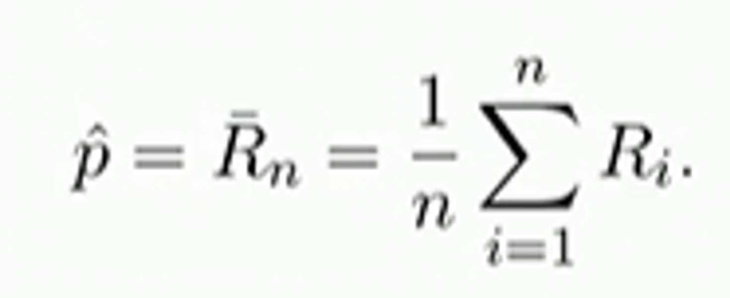
Formally, this procedure consists of doing the following:
- For i = 1, . . . ,n, define Ri = 1 if the ith couple turns to the right RIGHT, Ri = 0 otherwise.
- The estimator of $p$ is the
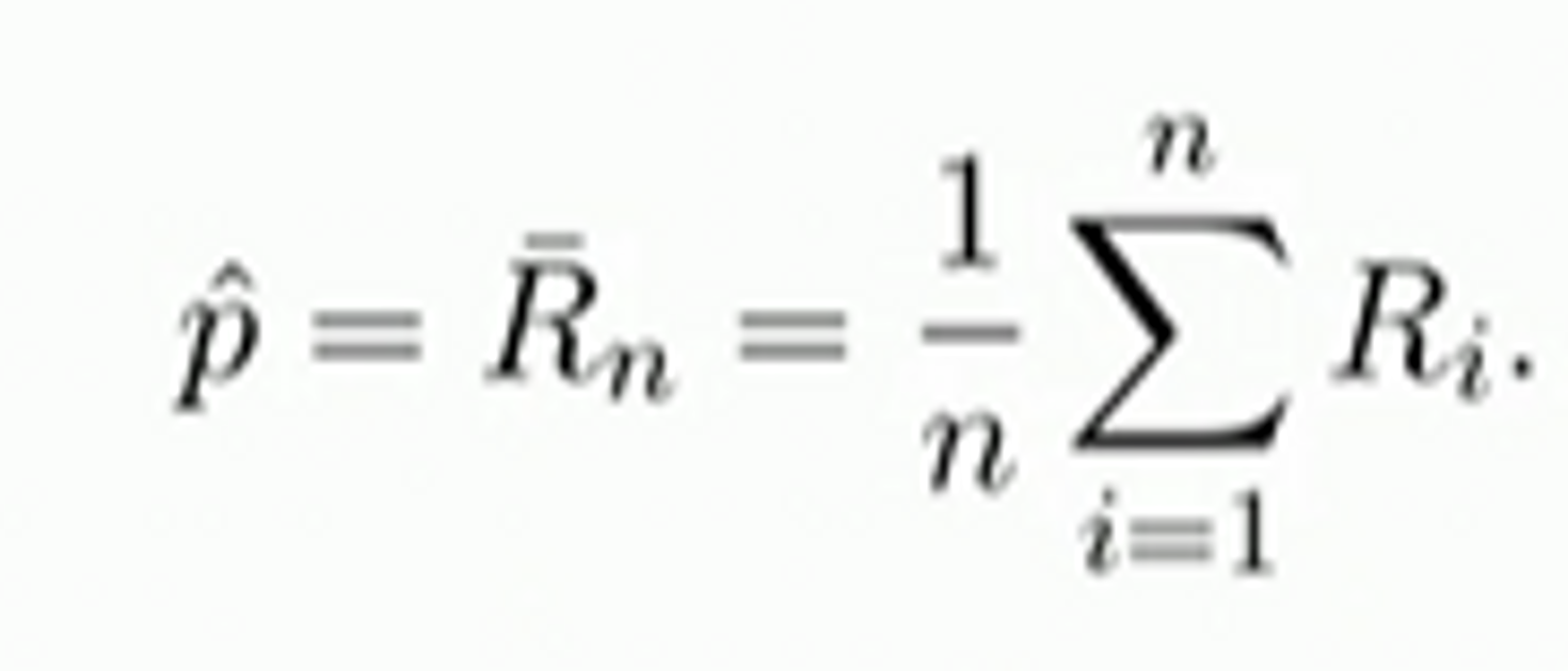
What is the accuracy of this estimator ?
In order to answer this question, we propose a statistical model that describes / approximates well the experiment. We think of the Ri’s as random variables so that p_hat is also a random variable. We need to understand its fluctuation.
Modelling assumptions
Coming up with a model consists of making assumptions on the observations Ri, i = 1, . . . ,n in order to draw statistical conclusions. Here are the assumptions we make:
- Each Ri is a random variable.
- Each of the r.v. Ri is Bernoulli with parameter p.
- R1, . . . ,Rn are mutually independent.
→ Ri 가 베르누이 분포를 따르는 이유는, Ri는 가질 수 있는 값이 0과 1, 즉, binary 값을 갖기 때문이다. 이렇게 p에 따라 두 개의 값을 가지는 확률 변수를 베르누이 분포를 따르는 확률변수라고 한다.
Let us discuss these assumptions
- Randomness is a way of modeling lack of information; with perfect information about the conditions of kissing (including what goes on in the kissers’ mind), physics or sociology would allow us to predict the outcome.
- Hence, the Ri’s are necessarily Bernoulli r.v. since Ri ∈ {0, 1}. They could still have a different parameter Ri ~ Ber(pi ) for each couple but we don’t have enough information with the data to estimate the pi’s accurately. So we simply assume that our observations come from the same process: pi = p for all i.
→ n개의 커플이 키스하는 방향(확률변수)이 똑같은 확률분포를 따를 것이라고 가정, pi는 p의 확률을 갖는 베르누이분포를 따름. - Independence is reasonable (people were observed at different locations and different times)
→ 플래시몹을 하지 않는 이상 공항에 있는 커플들이 동시에 갑자기 키스를 하지는 않을 것임. 따라서 커플들이 키스를 하는 행위를 독립 행위라 가정하자는 뜻
Population vs. Samples
- Assume that there is a total population of 5,000 “airport-kissing” couples
- Assume for the sake of argument that p = 35% or that p = 65%.
- What do samples of size 124 look like in each case?
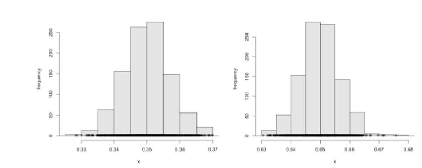
→ p와 1-p 어느쪽으로 histogram을 돌리던, 결과는 똑같다. 모수p를 기준으로, 정규분포 형태를 띄고 있음. 위 그림이 의미하는 것은, 키스를 하여 오른쪽으로 고개가 돌아갈 확률이 p인 베르누이 분포를 따르는 5000개 커플이 있을 때, 그 중 124개의 sample 만 뽑아서 확률 p_hat을 계산한 것.
Why probability?
We need to understand probabilistic aspects of the distribution of the random variable:
Specifically, we need to be able to answer questions such as:
- Is the expected value of p_hat close to the unknown p?
- Does p_hat take values close to p with high probability?
- Is the variance of p_hat large?
- I.e. does p_hat fluctuate a lot?
→ We need probabilistic tools! Most of them are about average of independent random variables.

'Statistics' 카테고리의 다른 글
| BDA 1 (0) | 2023.10.20 |
|---|---|
| 나아진다는 착각 (Why removing constants improves model performance) (0) | 2023.05.30 |
| Parametric Statistical Models (0) | 2023.02.19 |
| Probability Redux (1) | 2023.02.19 |